I enjoyed looking at the probabilistic model of world cup matches over at fivethirtyeight and was wondering how one would fare in terms of sports betting using the predictions from Nate Silver and Jay Boice. As a disclaimer: I did not bet any money at all, all of the below is purely theoretical.

So here is what I did: for each game, I pulled the winning probabilities from fivethirtyeight and the corresponding odds from online bookmakers. Since bookmakers constantly update their odds (in order to have an edge over bettors), I always pulled both probabilities and odds the night before the match. With that in hand, I simulated three different betting strategies. First, a bettor who always chooses the favorite to win. The second strategy is a contrarian bettor who always chooses the least likely outcome, which typically means betting on the underdog, but with high odds. Both of these strategies never adjust the size of their stake, and always bet 10% of their initial bankroll (not their current bankroll). Lastly, I will simulate a bettor that looks at all probabilities, and odds, and then uses the Kelly criterion for each bet. All bettors start out with the same bankroll of $100.

The Kelly criterion is a method to determine how much one should wager on a bet, given assumed winning probabilities, and offered odds. Kelly betting maximizes logarithmic utility. Below is a graphic display showing the Kelly criterion. On the x-axis are the probabilities that you assume an event is going to take place, and on the y-axis are the offered odds (these odds can be translated into implied probabilities of the bookie). The shading for each part of the graph shows what percentage of your current bankroll you should bet. As an example, if you believe the probability of an event to happen is close to 100% (right side of the graph), then you typically end up betting a lot (or all) of your bankroll (the yellow region of the graph). For events in which the implied probabilities of the bookie are larger than your own, you end up not betting at all - notice that this area is quite large in the graph.

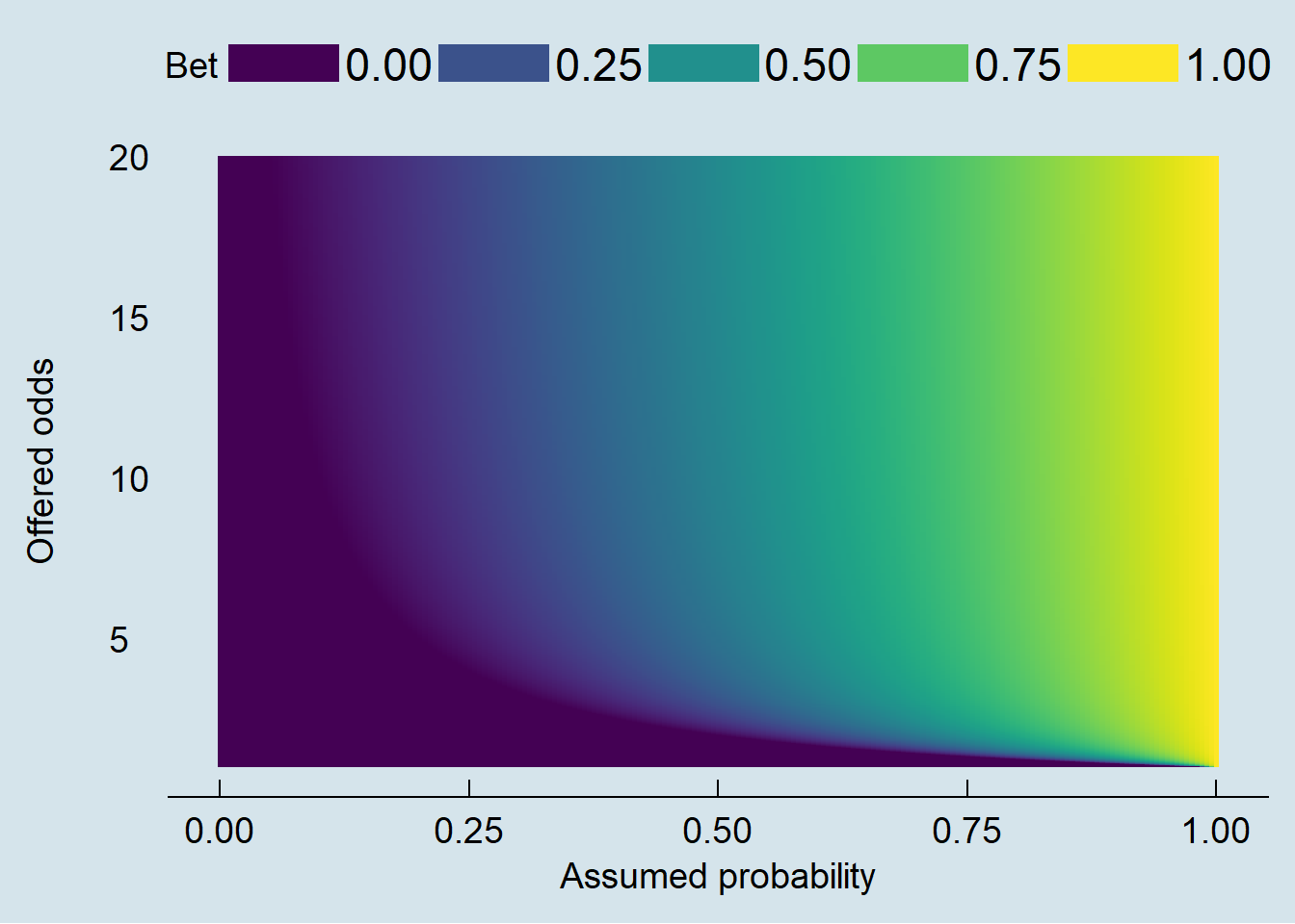
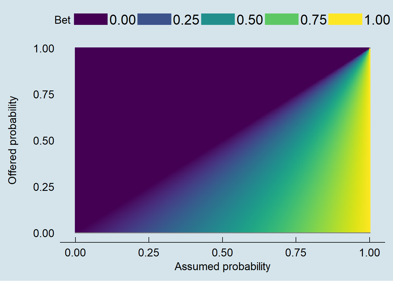
An interesting observation with respect to the World Cup games was that for many matches the Kelly criterion suggested not betting at all, especially not betting on the stronger team. This indicated that the offered odds from bookies generally tended to overestimate the winning probability (or maybe 538 underestimated the performance of strong teams). I should also add that I did not use the generalized Kelly criterion to distinguish the best bet between either team winning or a draw. I simply (and incorrectly) computed the Kelly bet for each outcome separately, and thus on occasion ended up with two outcomes that received a wager.

Below I am showing a linegraph that shows how the initial bankroll of $100 developed after each game. The y-axis shows relative bankroll (that means it simply tallies wins and losses and sets the zero point at the initial bankroll). The bars at the bottom of the graph show how much was won or lost in each bet, and the size of the point indicates the amount of total stake that was wagered on each game.

First, let’s have a look at the person who always bets on the favorite.

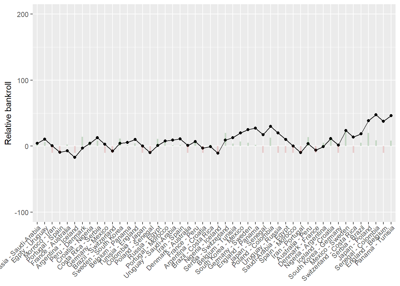We can see that basically two things happen: either the bettor loses the initial stake (which is always $10), or wins a modest amount (since odds for favorites are typically not very high). After the group stage this bettor still has managed to accumulate some winnings.

Comparing this with the contrarian bettor, we see a very different picture. This bettor is almost always losing the initial stake, and rarely wins. However the wins tend to be big. The largest gain was realized in the upset of South Korea over Germany. Without that single game, this bettor may be very close to bankruptcy already.

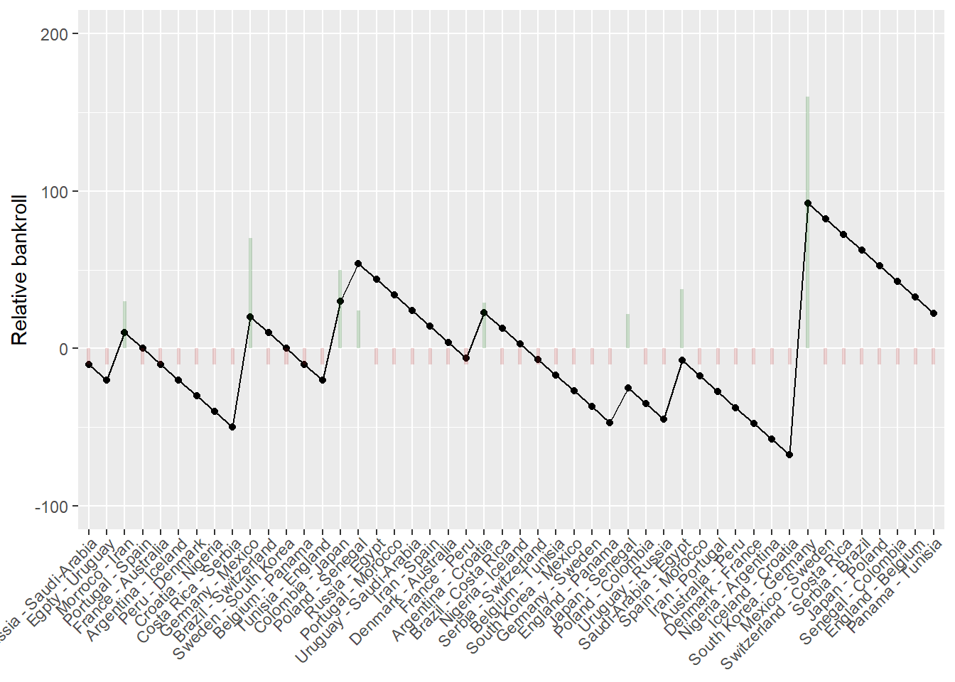
Finally, we look at the Kelly bettor, who only bets when the assumed probability of an outcome is higher than the implied probability of the bookmaker. This leads sometimes to bets on the favorite, but often on the underdog. In many instances, it also leads to not betting at all, or only using very small bets.

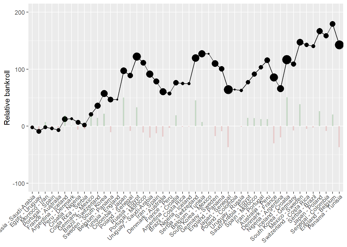
The Kelly bettor realized the largest winnings from all three strategies by a wide margin. At the end of the group stage, the Kelly bettor accumulated about $150 of winnings. It will be interesting to see how this developed in the knock-out stage.

library(ggplot2)
library(viridis)
library(ggthemes)
library(readxl)
library(dplyr)
library(magrittr)

prob <- seq(0,1,.005)
odds <- seq(1,20,.01)

grid <- expand.grid(prob=prob,odds=odds)

grid$kelley <- ((grid$odds*grid$prob)-1) / (grid$odds-1)
grid$kelley[grid$kelley<0] <- 0

ggplot(grid, aes(prob, odds, z = kelley)) +  
  geom_raster(aes(fill = kelley)) + scale_fill_viridis() + labs(x = "Assumed probability",  y= "Offered odds\n") +
  guides(fill = guide_legend(keywidth = 3, keyheight = 1, title="Bet")) + 
  theme_economist(base_size = 14) + theme(panel.border = element_blank(), panel.grid.major = element_blank(),
                     panel.grid.minor = element_blank(), axis.line = element_line(colour = "black"))



assumedprob <- seq(0,1,.005)

grid2 <- expand.grid(prob=prob,aprob=assumedprob)

grid2$kelley <- (((1/grid2$aprob)*grid2$prob)-1) / ((1/grid2$aprob)-1)
grid2$kelley[grid2$kelley<0] <- 0


ggplot(grid2, aes(prob, aprob, z = kelley)) +  
  geom_raster(aes(fill = kelley)) + scale_fill_viridis() + labs(x = "Assumed probability",  y= "Offered probability\n") +
  guides(fill = guide_legend(keywidth = 3, keyheight = 1, title="Bet")) + 
  theme_economist(base_size = 14) + theme(panel.border = element_blank(), panel.grid.major = element_blank(),
                                          panel.grid.minor = element_blank(), axis.line = element_line(colour = "black"))



#Data will be put on github, but only local for now
wcb <- read_xlsx("C:\\Users\\fjt36\\Dropbox\\WORK\\2018 Winter Cornell\\kellybettingwc.xlsx")
wcb <- wcb %>% mutate(posneg = factor(ifelse(wcb$`Total net`<0,"negative","positive"))) %>%  select(ID,Title,"Total net","Total stake",Bankrollkellyplot,posneg) %>% slice(1:13)

wcb$Title <- reorder(factor(wcb$Title),wcb$ID)

ggplot(wcb,aes(x=Title,y=Bankrollkellyplot-100)) + geom_point(aes(size=`Total stake`)) + geom_line(group=1) + theme(axis.text.x = element_text(angle=45,margin=margin(t=0,r=0,b=0,l=0),hjust=1)) +  geom_bar(data=wcb,aes(x=Title,y=`Total net`,fill=posneg),stat="identity",alpha=.2,width=.2) + scale_fill_manual(values=c("negative"="firebrick","positive"="darkgreen")) + ylab("Relative bankroll") +theme(axis.title.x=element_blank()) + guides(fill=FALSE,size=FALSE)

Back to posts